-
\( \require{cancel} \)
\( \require{colorv2} \)
- Types of ᖙᎯ𝜏ⲁ
- What is your favorite fruit?
- How many children do you have?
- How much puss came out when you squeezed that spot?
- ᑤᗗᖶᕨᘜᑸᓌᖇᓮᓧᕱᒹ ᗪᗩƬᎯ
-
ᑤᗗᖶᕨᘜᑸᓌᖇᓮᓧᕱᒹ ᖙᎯ𝜏ⲁ is when the answer isn't numerical:
What is your favorite fruit?
What mode of transport did you use to get to school today?
We could use a bar chart for this type of ᖙᎯ𝜏ⲁ, but it is more fun to use a pictogram:
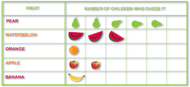
T.B.H, this type of ᖙᎯ𝜏ⲁ isn't particularly interesting to Mathematicians - because it ISN'T numerical and mathematicians can't draw pictures...
- Discrete ᗪᗩƬᎯ
-
Discrete usually means only integer-𝑣𝑎𝑙𝑢𝑒𝑠, but 🅽🅾🆃 always...
...for instance, shoe-sizes are discrete, but occupy whole numbers and half-numbers :
Shoe Sizes: 4, 4.5, 5, 5.5, 6, 6.5, 7, 7.5, 8, 8.5, 9, 9.5, 10 etc…
So are men's trouser's waist-sizes:
Waist Size: 28, 30, 32, 34, 36, 38, 40, 42, 44, 46 etc…
That said, \(99 \% \) of the time, discrete does mean integer-𝑣𝑎𝑙𝑢𝑒𝑠
(and often only natural numbers...)Discrete ᖙᎯ𝜏ⲁ can be given as a ᒺᓲᔜᖶ of ᖙᎯ𝜏ⲁ, like this:
Shoe Sizes: 4, 4.5, 5, 5.5, 6, 6.5, 7, 7.5, 8, 8.5, 9, 9.5, 10 etc…
Or, as a ᖶᕬᙗᒶᕦ of un-grouped ᖙᎯ𝜏ⲁ
Shoe Size𝑓𝑟𝑒𝑞𝑢𝑒𝑛𝑐𝑦5261071881595Do 🅽🅾🆃 use a 𝓬𝓾𝓶𝓾𝓵𝓪𝓽𝓲𝓿𝓮-𝓯𝓻𝓮𝓺𝓾𝓮𝓷𝓬𝔂 𝓬𝓾𝓻𝓿𝓮
for discrete, un-grouped ᖙᎯ𝜏ⲁBut, discrete ᖙᎯ𝜏ⲁ can also be given as a ᖶᕬᙗᒶᕦ of ցɾσᥙρҽԃ ᖙᎯ𝜏ⲁ:
№ of errors𝑓𝑟𝑒𝑞𝑢𝑒𝑛𝑐𝑦0 – 5105 – 787 – 9149 – 111211 – 151615 – 2020Once discrete ᖙᎯ𝜏ⲁ has been ցɾσᥙρҽԃ, we kinda gotta treat it as 𝒸ℴ𝓃𝓉𝒾𝓃𝓊ℴ𝓊𝓈
- 𝓒ℴ𝓃𝓉𝒾𝓃𝓊ℴ𝓊𝓈 ᗪᗩƬᎯ
-
𝓒ℴ𝓃𝓉𝒾𝓃𝓊ℴ𝓊𝓈 ᖙᎯ𝜏ⲁ usually means things that you have to measure...
Clearly, a feature of a 𝒸ℴ𝓃𝓉𝒾𝓃𝓊ℴ𝓊𝓈 variable is that you can you can never measure it to \(100 \%\) accuracy: You'll have to decide whether to to give it to (say) \(3\) s.f. or (say) \(5\) s.f. etc...
Discrete𝒱 𝓒ℴ𝓃𝓉𝒾𝓃𝓊ℴ𝓊𝓈
So, the PROPER TEST to decide if ᖙᎯ𝜏ⲁ is discrete or not, is this:
Pick two possible answers to the question (e.g. I'm shoe size ‘8½’, my brother is shoe size ‘10’)
Is it possible to find an answer that is BETWEEN those answers?
YES: Shoe-size ‘9’ is between shoe-size ‘8½’ and shoe-size ‘10’
Now, arks yourself again, is it possible to find an answer BETWEEN the closest pair?
Well, the closest pair out of ‘8½’, ‘9’ and ‘10’ is: ‘8½’ & ‘9’
NO: There is no shoe-size between shoe-sizes ‘8½’ and ‘9’
So, with discrete ᖙᎯ𝜏ⲁ, you'll eventually find a pair of numbers that are so close together, that it is impossible to find an answer BETWEEN them (that will never happen for 𝒸ℴ𝓃𝓉𝒾𝓃𝓊ℴ𝓊𝓈 ᖙᎯ𝜏ⲁ...)
- 𝓒𝓾𝓶𝓾𝓵𝓪𝓽𝓲𝓿𝓮-𝓯𝓻𝓮𝓺𝓾𝓮𝓷𝓬𝔂 𝓬𝓾𝓻𝓿𝓮
- Check the ᖙᎯ𝜏ⲁ is written using ᙅしᗩ⟆⟆-ᗷ〇⋃Ɲᗩᗪᖇᓮᕮ⟆ (NOT ⊂Լᗩ𝛓Ϩ-し⫯ᵐ𝒾𝜏⟆ - YUK!)
- Write a ᖶᕬᙗᒶᕦ of 𝓬𝓾𝓶𝓾𝓵𝓪𝓽𝓲𝓿𝓮-𝓯𝓻𝓮𝓺𝓾𝓮𝓷𝓬𝓲𝓮𝓼
- Pull out your pad of graph paper, plot an O̷G̷I̷V̷E̷ (i.e. a 𝓬𝓾𝓶𝓾𝓵𝓪𝓽𝓲𝓿𝓮-𝓯𝓻𝓮𝓺𝓾𝓮𝓷𝓬𝔂 𝓬𝓾𝓻𝓿𝓮 )
- To find \(n\left( X \lt a \right) \) (the number of ᖙᎯ𝜏ⲁ items below \(a\) ), add a vertical line at \(X = a\): Once it meets the O̷G̷I̷V̷E̷, change to a horizontal line - where that meets the \(y\)-axis gives you \(n\left( X \lt a \right) \)
- To find \(n\left( X \gt b \right) \) (the number of ᖙᎯ𝜏ⲁ items above \(b\) ), simply calculate: \(\Large{n}\) \(-\) \(n\left( X \lt a \right) \)
- To find \(n\left( a \lt X \lt b \right) \) (the number of ᖙᎯ𝜏ⲁ items between \(a\) and \(b\) ), simply subtract: \(n\left( X \lt b \right) - n\left( X \lt a \right)\)
- Draw a vertical-line starting a \(\color{var(--midgreen)}{x=22}\)
- Where that line meets the curve, mark a ○
- Next, from the ○ you marked, draw a horizontal-line to the \(\color{var(--midblue)}{y}\)-axis
- The number you read off the \(\color{var(--blue)}{y}\)-axis tells you \(n\left( X \lt 22 \right) \) (the number of pupils that got less than \(22\) marks )
- Draw a vertical-line starting a \(\color{var(--midgreen)}{x=22}\)
- Where that line meets the curve, draw a horizontal-line to the \(\color{var(--midblue)}{y}\)-axis
- The number you read off the \(\color{var(--blue)}{y}\)-axis tells you \(n\left( X \lt 22 \right) \) (the number of pupils that scored less than \(22\) ) marks
- If you want: \(n\left( X \gt 22 \right) \) marks (№ of pupils that scored more than \(22\) ) marks; subtract the previous answer from ❛\(\color{var(--red)}{n=100}\)❜
- Draw two vertical-lines at \(\color{var(--midgreen)}{x=27}\) and at \(\color{var(--midgreen)}{x=22}\)
- Where each line meets the curve, draw a horizontal-line to the \(\color{var(--midblue)}{y}\)-axis
- The numbers you read off the \(\color{var(--blue)}{y}\)-axis tells you \(n\left( X \lt 27 \right) \) and \(n\left( X \lt 22 \right) \)
- To find: \(n\left(22 \lt X \lt 27 \right) \) marks simply subtract these two \(\color{var(--blue)}{y}\)-values
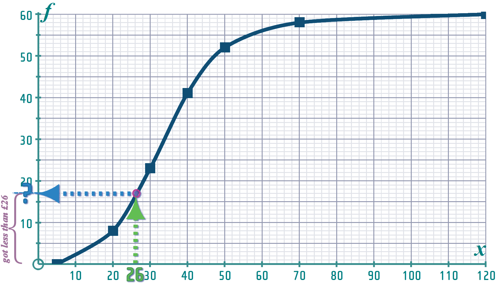
- Draw a vertical-line starting a \(\color{var(--midgreen)}{x=26}\)
- Where that line meets the curve, mark a ○
- Next, from the ○ you marked, draw a horizontal-line to the \(\color{var(--midblue)}{y}\)-axis
- The number you read off the \(\color{var(--blue)}{y}\)-axis tells you \(n\left( X \lt £26 \right) \) (the number of pupils that got less than \(£26\) )
- If you want: \(n\left( X \gt £26 \right) \) (the number of pupils that got more than \(£26\) ) simply subtract the previous answer from ❛\(\color{var(--red)}{60}\)❜
- Draw a vertical-line starting a \(\color{var(--midgreen)}{x=16.25}\)
- Where that line meets the curve, mark a ○
- Next, from the ○ you marked, draw a horizontal-line to the \(\color{var(--midblue)}{y}\)-axis
- The number you read off the \(\color{var(--blue)}{y}\)-axis tells you \(n\left( X \lt £16.25 \right) \) (the number of pupils that got less than \(£16.25\) )
- If you want: \(n\left( X \gt £16.25 \right) \) (the number of pupils that got more than \(£16.25\) ) simply subtract the previous answer from ❛\(\color{var(--red)}{60}\)❜
- Draw two vertical-lines at \(\color{var(--midgreen)}{x=45.00}\) and at \(\color{var(--midgreen)}{x=32.50}\)
- Where each line meets the curve, draw a horizontal-line to the \(\color{var(--midblue)}{y}\)-axis
- The numbers you read off the \(\color{var(--blue)}{y}\)-axis tells you \(n\left( X \lt £45.00 \right) \) and \(n\left( X \lt £32.50 \right) \)
- To find: \(n\left(£32.50 \lt X \lt £45.00 \right) \) simply subtract these two \(\color{var(--blue)}{y}\)-values
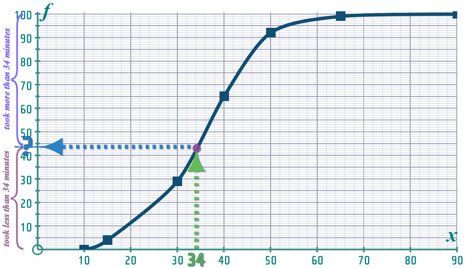
- Draw a vertical-line starting a \(\color{var(--midgreen)}{x=34}\)
- Where that line meets the curve, mark a ○
- Next, from the ○ you marked, draw a horizontal-line to the \(\color{var(--midblue)}{y}\)-axis
- The number you read off the \(\color{var(--blue)}{y}\)-axis tells you \(n\left( X \lt £34 \right) \) (the number of competitors that took less than \(34\) minutes )
- We want: \(n\left( X \gt 34 \right) \) (the number of competitors that took longer than \(34\) minutes ), so simply subtract the previous answer from ❛\(\color{var(--red)}{100}\)❜
- Draw a horizontal-line starting at \(\color{var(--midblue)}{y = 38}\)
- Where that line meets the curve, mark a ○
- Next, from the ○ you marked, draw a vertical-line down to the \(\color{var(--midgreen)}{x}\)-axis
- The value you read off the \(\color{var(--midgreen)}{x}\)-axis tells you \(m_c\), solving \(n\left( X \lt m_c \right) = 38\) (bags less than \(m_c\) kg won't get dumped )
- ⲙⲉᕍ╹ⲓⲁⲛ and ႳⴑⲀꞄⲦⲒ𝓛ⲈϨ
- \(25 \%\) of the ᖙᎯ𝜏ⲁ is values below \(Ⴓ_{1}\) (this is the left-tail of the distribution)
- \(50 \%\) of the ᖙᎯ𝜏ⲁ is between \(Ⴓ_{1}\) and \(Ⴓ_{3}\) (this is the central-part of the ᖙᎯ𝜏ⲁ)
- \(25 \%\) of the ᖙᎯ𝜏ⲁ is values above \(Ⴓ_{3}\) (this is the right-tail of the distribution)
- The ⲙⲉᕍ╹ⲓⲁⲛ (\(Ⴓ_{2}\)) is the \(\left( \frac{1}{2}n + \frac{1}{2} \right) \)th-𝑣𝑎𝑙𝑢𝑒 (or the \(\frac{1}{2}n\)th-𝑣𝑎𝑙𝑢𝑒, if \(n>30\) )
- The ႳⴑⲀꞄⲦⲒ𝓛ⲈϨ are the \(\left( \frac{1}{4}n + \frac{1}{2} \right) \)th- and \(\left( \frac{3}{4}n + \frac{1}{2} \right) \)-𝑣𝑎𝑙𝑢𝑒𝑠 (If \(n>30\); the \(\frac{1}{4}n\)th- and \(\frac{3}{4}n\)th-𝑣𝑎𝑙𝑢𝑒𝑠)
- Look up those 𝑣𝑎𝑙𝑢𝑒𝑠 on the \(y\)-axis, then across to the curve, then read down to the \(x\)-axis
- ᖘᕮᖇᑕᕮƝƬᓮしᕮ⟆
- ᖘᕮᖇᑕᕮƝƬᓮしᕮ⟆ are just like ႳⴑⲀꞄⲦⲒ𝓛ⲈϨ (except there are more of them...)
- To find the \(90\)th ᖘᕮᖇᑕᕮƝƬᓮしᕮ, calculate \(\frac{90}{100}n\)
- Look up those 𝑣𝑎𝑙𝑢𝑒𝑠 on the \(y\)-axis, then across to the curve, then read down to the \(x\)-axis
- The 𝕀ƝƬⲈꞄᖘᕮᖇᑕᕮƝƬᓮしᕮ-ᖇᗩƝᎶⲈ (\(ᖘ_{90} - ᖘ_{10}\)) is used when it's not possible to find the ᖇᗩƝᎶᕮ
Cumulative Frequency Curves
When we collect ᖙᎯ𝜏ⲁ, we usually ask a question:
OR
OR
The answers we get will tell us if the ᖙᎯ𝜏ⲁ is ❛ categorical-ᖙᎯ𝜏ⲁ ❜, ❛ discrete ᖙᎯ𝜏ⲁ ❜ or ❛ 𝒸ℴ𝓃𝓉𝒾𝓃𝓊ℴ𝓊𝓈 ᖙᎯ𝜏ⲁ ❜
𝓒ℴ𝓃𝓉𝒾𝓃𝓊ℴ𝓊𝓈 ᖙᎯ𝜏ⲁ Ⲁ𝓛ⲰⲀⲨϨ has to be ցɾσᥙρҽԃ
We already know how to represent ցɾσᥙρҽԃ ᖙᎯ𝜏ⲁ using a ▁▆▇▅▙▂ Ԩ⫯⟆𝜏〇ɢᖇᎯⲙ
Another way of representing ցɾσᥙρҽԃ ᖙᎯ𝜏ⲁ is to draw a 𝓬𝓾𝓶𝓾𝓵𝓪𝓽𝓲𝓿𝓮-𝓯𝓻𝓮𝓺𝓾𝓮𝓷𝓬𝔂 𝓬𝓾𝓻𝓿𝓮
(also called an O̷G̷I̷V̷E̷)
If you're give a set of ցɾσᥙρҽԃ ᖙᎯ𝜏ⲁ (discrete or 𝒸ℴ𝓃𝓉𝒾𝓃𝓊ℴ𝓊𝓈), then you can find \(n\left( X \lt a \right) \) (the number of ᖙᎯ𝜏ⲁ items below \(a\) ) or \(n\left( X \gt b \right) \) (the number of ᖙᎯ𝜏ⲁ items above \(b\) )...
...and you can also find the ⲙⲉᕍⲓⲁⲛ and ႳⴑⲀꞄⲦⲒ𝓛ⲈϨ:
This will deliver estimates of, \(n\left( X \lt a \right) \), \(n\left( X \gt b \right) \) and \(n\left( a \lt X \lt b \right) \)
\(100\) A-level pupils are given a test (out of 30 marks). The table below summarises their reuslts
Using an O̷G̷I̷V̷E̷ , estimate how many pupils got:
(a) less than \(22\) marks
(b) more than \(22\) marks
(c) Between \(22\) and \(27\) marks
#1 » Check it's written using: ᙅしᗩ⟆⟆-ᗷ〇⋃Ɲᗩᗪᖇᓮᕮ⟆
            ╒════════════╕   ╒═════════╕ ╖
             NO gap between                 And start           ╟ This is written using
              end of 1st class                of 2nd class           ╟ ❛ ᙅしᗩ⟆⟆-ᗷ〇⋃Ɲᗩᗪᖇᓮᕮ⟆ ❜
            ╘══════════╦═╛   ╘═╦═══════╛ ╜
                       ▼       ▼
#2 » Form a TABLE of 𝓬𝓾𝓶𝓾𝓵𝓪𝓽𝓲𝓿𝓮-𝓯𝓻𝓮𝓺𝓾𝓮𝓷𝓬𝓲𝓮𝓼
Start with the L.C.B. of the \(1^{st}\)-𝒞ℒ𝒜𝒮𝒮...
...after that, use the U.C.B.s of ALL of the other 𝒞ℒ𝒜𝒮𝒮ℰ𝒮:
                  ┌─Place these 𝑣𝑎𝑙𝑢𝑒𝑠 in the ⲦⲞⲢ-ꞄⲞⲰ of a 𝓬𝓾𝓶𝓾𝓵𝓪𝓽𝓲𝓿𝓮-𝓯𝓻𝓮𝓺𝓾𝓮𝓷𝓬𝔂 𝚃𝙰𝙱𝙻𝙴    │           │           │             │            │           ─┐
                  │     │           │           │             │            │            │
                  ▼     ▼           ▼           ▼             ▼            ▼            ▼
Fill in the \(2^{nd}\) ꞄⲞⲰ, start with a first value of \(\color{var(--)}{0}\), and the the running total of the 𝓯𝓻𝓮𝓺𝓾𝓮𝓷𝓬𝓲𝓮𝓼
              ▲           ▲           ▲           ▲
𝒜ℒℒ  Ƒ-𝚃𝙰𝙱𝙻𝙴𝚂              │           │           │           │          ETC         ETC
start from ZERO             ─┘        ┌──┴──┐     ┌──┴──┐    ┌───┴───┐
                       │ just 4     │     │ 4 + 18     │    │4+18+22       │
                       └─────┘     └─────┘    └───────┘
#3 » Plot the points and connect with a 𝓼̷𝓶̷𝓸̷𝓸̷𝓽̷𝓱̷ ?-curve (the O̷G̷I̷V̷E̷ )
Connect these points with a 𝓼̷𝓶̷𝓸̷𝓸̷𝓽̷𝓱̷ -curve that starts from the origin and ends flat & horizontal (after the last point):
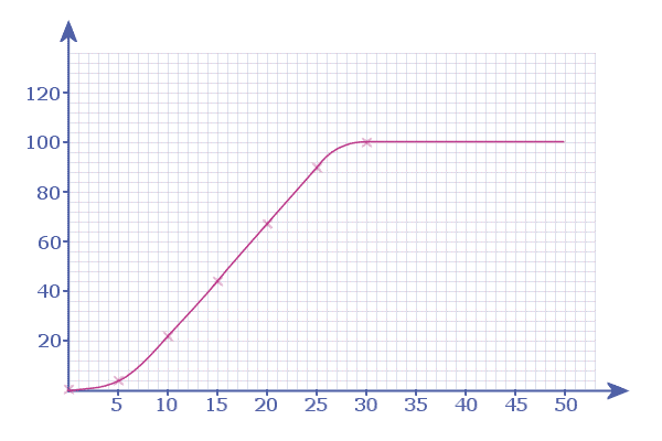
The last number on the 𝓬𝓾𝓶𝓾𝓵𝓪𝓽𝓲𝓿𝓮-𝓯𝓻𝓮𝓺𝓾𝓮𝓷𝓬𝔂 table is \(\color{var(--red)}{n=100}\)
Part (a):
To find the number of pupils who scored less than \(22\) marks i.e. \(n\left( X \lt 22 \right) \) :
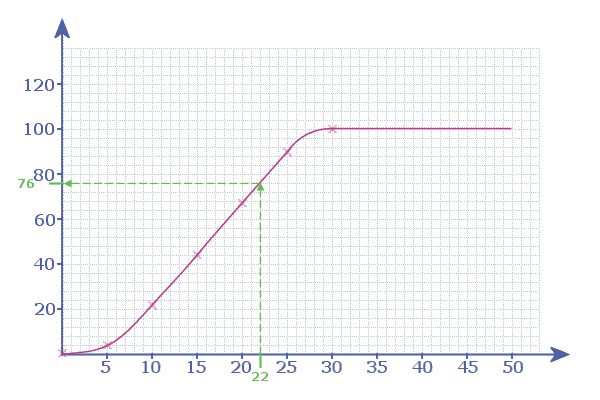
Which shows that \(\color{var(--blue)}{76}\) pupils scored less than \(\color{var(--midgreen)}{22}\) marks
Part (b):
To find the number of pupils who scored more than \(22\) marks i.e. \(n\left( X \gt 22 \right) \) :
Which shows that \(\color{var(--blue)}{24}\) pupils scored more than \(\color{var(--midgreen)}{22}\) marks
Part (c):
To find the number of pupils who scored between \(22\) and \(27\) marks i.e. \(n\left( 22 \lt X \lt 27 \right) \) :
(Don't round before subtracting, but if after subtracting the answer ISN'T a whole number, round it DOWN)
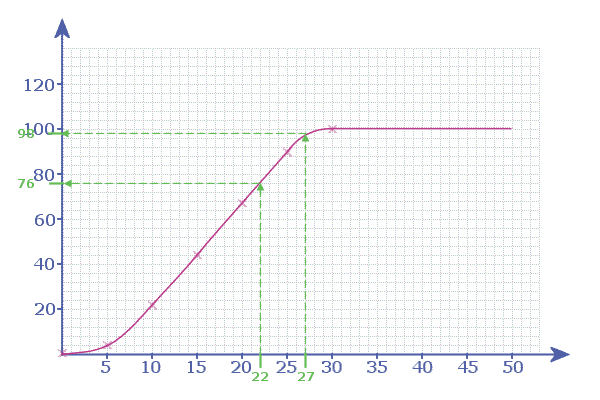
Which shows that \(\color{var(--blue)}{22}\) pupils scored between \(\color{var(--midgreen)}{22}\) and \(\color{var(--midgreen)}{27}\) marks
In this Web Lesson, you'll see links for grids:
Print them off and use them to answer the questions
Alternatively, click HERE to download all the links in one go!
A class of 60 pupils were asked how much Christmas money they received
The results are given in this table:
a) Complete the following cumulative frequency table for these ᖙᎯ𝜏ⲁ:
b) Using the GRID linked here, sketch the 𝓬𝓾𝓶𝓾𝓵𝓪𝓽𝓲𝓿𝓮-𝓯𝓻𝓮𝓺𝓾𝓮𝓷𝓬𝔂 𝓬𝓾𝓻𝓿𝓮 for these ᖙᎯ𝜏ⲁ
c) Using your curve, estimate how many students got:
(i) less than \(£26.00\)
(ii) more than \(£16.25\)
(iii) Between \(£32.50\) and \(£45.00\)
CLARIFICATION: In this web lesson, you see classes written in the form: \(5-20\)
...which is just an abbreviated way of saying: \(5\leqslant x<20\)
Hint
Before we do anything else - the first thing we need to do is:
#1 » Check it's written using: ᙅしᗩ⟆⟆-ᗷ〇⋃Ɲᗩᗪᖇᓮᕮ⟆
            ╒════════════╕   ╒═════════╕ ╖
             NO gap between                 And start           ╟ This is written using
              end of 1st class                of 2nd class           ╟ ❛ ᙅしᗩ⟆⟆-ᗷ〇⋃Ɲᗩᗪᖇᓮᕮ⟆ ❜
            ╘══════════╦═╛   ╘═╦═══════╛ ╜
                       ▼       ▼
Great - so no issue there...
...we can move on:
Part (a):
#2 » Form a TABLE of 𝓬𝓾𝓶𝓾𝓵𝓪𝓽𝓲𝓿𝓮-𝓯𝓻𝓮𝓺𝓾𝓮𝓷𝓬𝓲𝓮𝓼
Start with the L.C.B. of the \(1^{st}\)-𝒞ℒ𝒜𝒮𝒮...
...after that, use the U.C.B.s of ALL of the other 𝒞ℒ𝒜𝒮𝒮ℰ𝒮:
                  ┌─ Place these 𝑣𝑎𝑙𝑢𝑒𝑠 in the ⲦⲞⲢ-ꞄⲞⲰ of a 𝓬𝓾𝓶𝓾𝓵𝓪𝓽𝓲𝓿𝓮-𝓯𝓻𝓮𝓺𝓾𝓮𝓷𝓬𝔂 𝚃𝙰𝙱𝙻𝙴    │           │            │            │            │          ─┐
                  │     │           │            │            │            │           │
                  ▼     ▼           ▼            ▼            ▼            ▼           ▼
Fill in the \(2^{nd}\) ꞄⲞⲰ, start with a first value of \(\color{var(--orange)}{0}\), and then, the running total of the 𝓯𝓻𝓮𝓺𝓾𝓮𝓷𝓬𝓲𝓮𝓼
              ▲           ▲           ▲           ▲           ▲           ▲           ▲
𝒜ℒℒ  Ƒ-𝚃𝙰𝙱𝙻𝙴𝚂              │           │           │           │          ETC         ETC         ETC
start from ZERO             ─┘        ┌──┴──┐     ┌──┴──┐    ┌───┴───┐
                       │ just 8     │     │ 8 + 15     │    │8+15+18       │
                       └─────┘     └─────┘    └───────┘
Part (b):
#3 » Plot the points and connect with a 𝓼̷𝓶̷𝓸̷𝓸̷𝓽̷𝓱̷ -curve (the O̷G̷I̷V̷E̷ )
PRINT off this GRID: Plot the points and connect the points with a 𝓼̷𝓶̷𝓸̷𝓸̷𝓽̷𝓱̷ -curve that starts from the origin and ends flat & horizontal (after the last point):
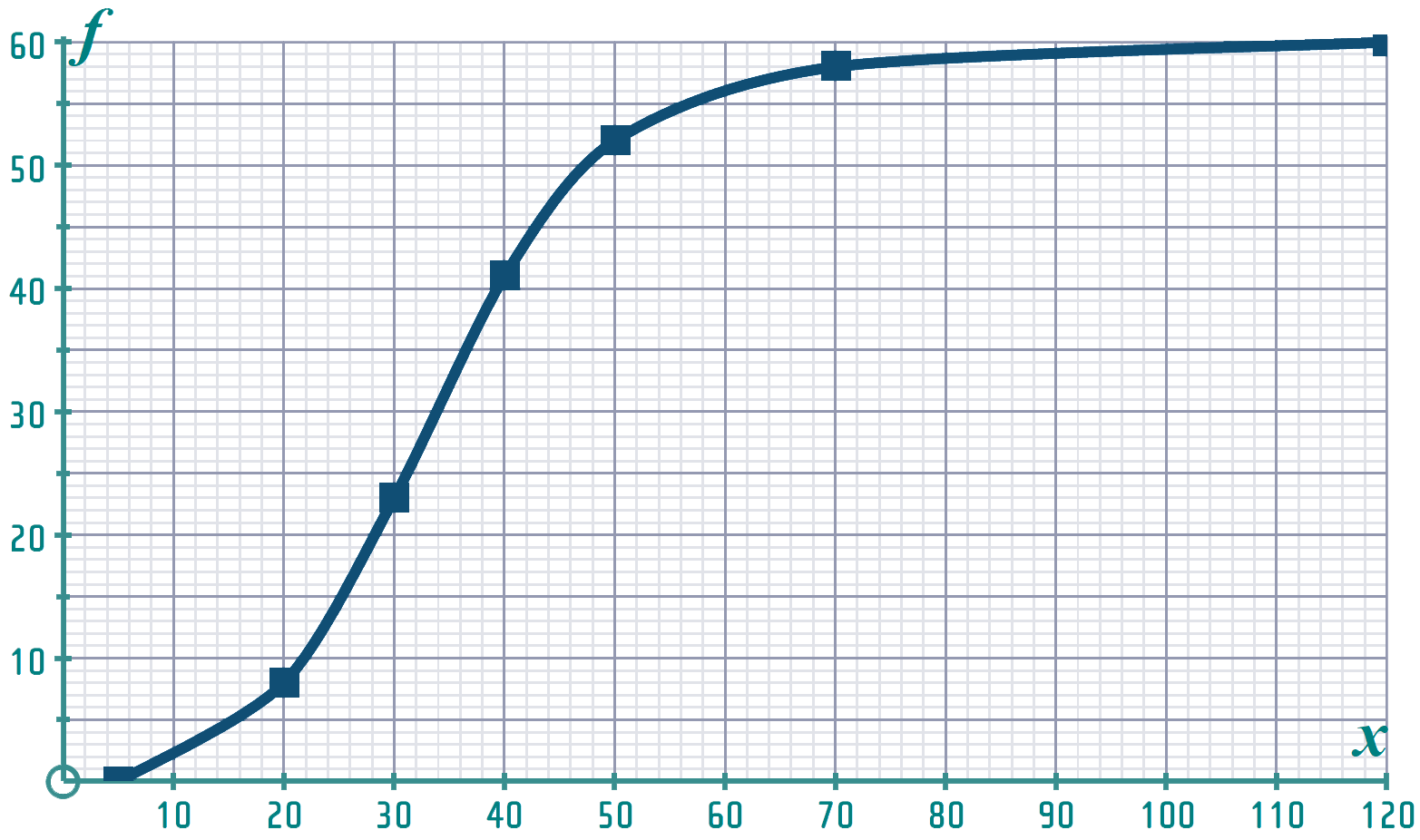
Part (ci):
To find the number of pupils who got less than \(£26\) i.e. \(n\left( X \lt £26 \right) \) :
(If you start with \(\color{var(--midgreen)}{x=£36}\), you get \(\color{var(--blue)}{y=33.8}\), which is NOT a whole number: We'd round it DOWN, so \(n\left( X \lt £36 \right) = 33\)
Part (cii):
To find the number of pupils who got more than \(£16.25\) i.e. \(n\left( X \gt £16.25 \right) \) :
(If you start with \(\color{var(--midgreen)}{x=£36}\), you get \(\color{var(--blue)}{y=33.8}\), which is NOT a whole number: We round it DOWN, so \(n\left( X \lt £36 \right) = 33\)
Part (ciii):
To find the number of pupils who got between \(£32.50\) and \(£45.00\) i.e. \(n\left( £32.50 \lt X \lt £45.00 \right) \) :
(Don't round before subtracting, but if after subtracting the answer ISN'T a whole number, round it DOWN)
Some ᖙᎯ𝜏ⲁ was collected on the time taken to complete a crossword (with a 2-minute penalty for each incomplete/incorrect entry) in Round 1 of a competition:
a) Form a cumulative frequency table for these ᖙᎯ𝜏ⲁ
b) Using the GRID linked here, sketch the Cumulative Frequency Curve for these ᖙᎯ𝜏ⲁ
Competitors that took longer than 34 minutes were eliminated and did not go through to Round 2
c) What proportion were eliminated in Round 1
Hint
Before we do anything else - the first thing we need to do is:
#1 » Check it's written using: ᙅしᗩ⟆⟆-ᗷ〇⋃Ɲᗩᗪᖇᓮᕮ⟆
            ╒════════════╕   ╒═════════╕ ╖
             NO gap between                 And start           ╟ This is written using
              end of 1st class                of 2nd class           ╟ ❛ ᙅしᗩ⟆⟆-ᗷ〇⋃Ɲᗩᗪᖇᓮᕮ⟆ ❜
            ╘══════════╦═╛   ╘═╦═══════╛ ╜
                       ▼       ▼
Great - so no issue there...
...we can move on:
Part (a):
#2 » Form a TABLE of 𝓬𝓾𝓶𝓾𝓵𝓪𝓽𝓲𝓿𝓮-𝓯𝓻𝓮𝓺𝓾𝓮𝓷𝓬𝓲𝓮𝓼
Start with the L.C.B. of the \(1^{st}\)-𝒞ℒ𝒜𝒮𝒮...
...after that, use the U.C.B.s of ALL of the other 𝒞ℒ𝒜𝒮𝒮ℰ𝒮:
                  ┌─ Place these 𝑣𝑎𝑙𝑢𝑒𝑠 in the ⲦⲞⲢ-ꞄⲞⲰ of a 𝓬𝓾𝓶𝓾𝓵𝓪𝓽𝓲𝓿𝓮-𝓯𝓻𝓮𝓺𝓾𝓮𝓷𝓬𝔂 𝚃𝙰𝙱𝙻𝙴    │           │            │            │            │          ─┐
                  │     │           │            │            │            │           │
                  ▼     ▼           ▼            ▼            ▼            ▼           ▼
Fill in the \(2^{nd}\) ꞄⲞⲰ, start with a first value of \(\color{var(--orange)}{0}\), and then, the running total of the 𝓯𝓻𝓮𝓺𝓾𝓮𝓷𝓬𝓲𝓮𝓼
              ▲           ▲           ▲           ▲           ▲           ▲           ▲
𝒜ℒℒ  Ƒ-𝚃𝙰𝙱𝙻𝙴𝚂              │           │           │           │          ETC         ETC         ETC
start from ZERO             ─┘        ┌──┴──┐     ┌──┴──┐    ┌───┴───┐
                       │ just 4     │     │ 4 + 25     │    │4+25+36       │
                       └─────┘     └─────┘    └───────┘
Part (b):
#3 » Plot the points and connect with a 𝓼̷𝓶̷𝓸̷𝓸̷𝓽̷𝓱̷ -curve (the O̷G̷I̷V̷E̷ )
PRINT off this GRID: Plot the points and connect the points with a 𝓼̷𝓶̷𝓸̷𝓸̷𝓽̷𝓱̷ -curve that starts from the origin and ends flat & horizontal (after the last point):
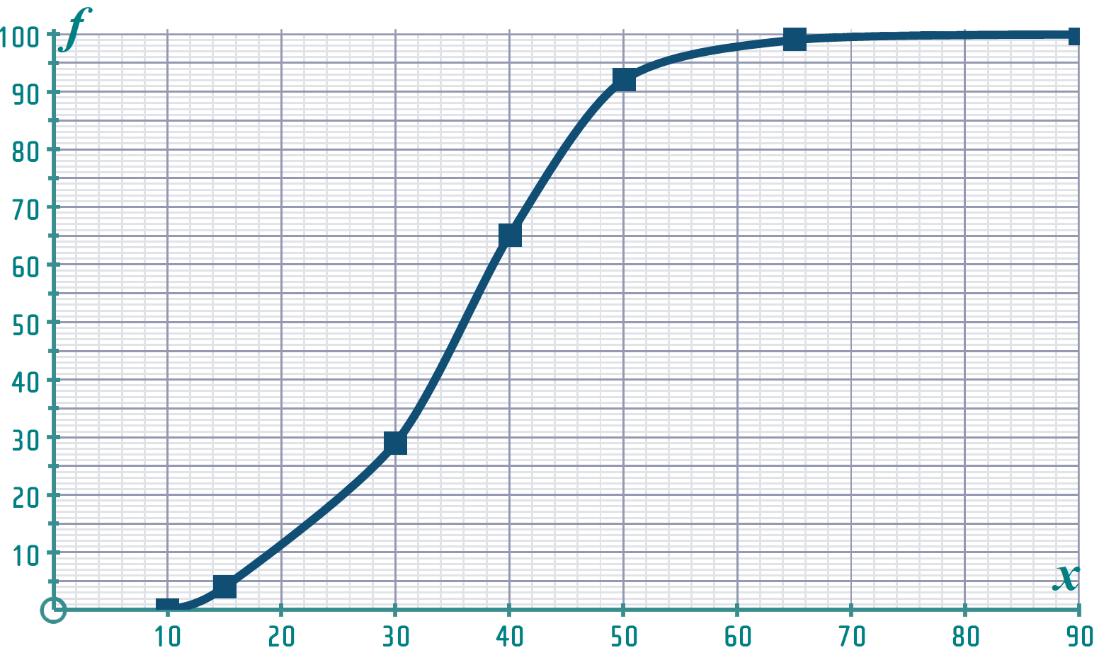
Part (c):
To find the number of competitors who took longer than \(34\) minutes i.e. \(n\left( X \gt 34 \right) \) :
(\(\color{var(--midgreen)}{x=34}\), doesn't yield an integer-value of \(\color{var(--blue)}{y}\); so round DOWN by reading the INTEGER \(\color{var(--midblue)}{y}\)-value just below your horizontal-line)
Indian airlines tells its passengers that they can "carry on" hand baggage of up to \(10\) kg, but anything above \(10\) kg has to be checked into the hold and the customer needs to PAY for it.
On Tuesday's flight, 48 people tried to board the plane with OVERWEIGHT hand-baggage. This table summarises the masses of those idiots (well, their bags)
a) Complete a Cumulative Frequency table for these ᖙᎯ𝜏ⲁ
b) Using the GRID linked here, sketch the Cumulative Frequency Curve for these ᖙᎯ𝜏ⲁ
It is decided to teach everyone on the flight a lesson: So an announcement is made durning the flight
Those of you with heavy bags: The \(10\) heaviest are going to be ejected from the plane.
c) I'm scared - my bag weighed \(£23.5\) kg. Is my bag going to be dumped from the plane?
Hint
Hints & helpful advice:
Part (a):
Don't start your cumulative frequency curve from the point \(\left( 0,0 \right) \)
As we have done in the questions so far, this time, you have to start from the point \(\left( \text{L.C.L. of 1ˢᵗ class}, 0 \right) \)
Part (c):
This is effectively the REVERSE of what we had to do in Part (c) of the previous questions: They TELL us the \(10\) heaviest bags are to be ejected (i.e. the other \(48\) bags are less than whatever critical mass (\(m_c\)) is above which your bag is history). So: \(n ( X \lt \underbrace{m_{c}}_{\scriptsize{\substack{\text{we don't} \\ \text{know this} }}} ) = 38\)
To find the mass that \(38\) bags were less than i.e. Solve: \(n\left( X \lt m_c \right) = 38\) :
The ⲙⲉᕍ╹ⲓⲁⲛ (\(Ⴓ_{2}\)) and the ႳⴑⲀꞄⲦⲒ𝓛ⲈϨ (\(Ⴓ_{1}\) and \(Ⴓ_{3}\)) are related to probability:
For instance, if you think about adult female B.M.I, you might say that those with particularly low BMI (below \(Ⴓ_{1} = 18.5\)) are underweight...
Those with a normal BMI (between \(Ⴓ_{1} = 18.5\) and \(Ⴓ_{3} = 25\)) are at in the heathly weight-range
Those with a high B.M.I. (above \(Ⴓ_{3} = 25\)) are overweight and that might have some health implications...
So it is a very simple way if dividing up a ᖙᎯ𝜏ⲁ set...
In the Web Lesson, we looked at some ᖙᎯ𝜏ⲁ distance the Javelin was thrown by Cündi
Find the ⲙⲉᕍ╹ⲓⲁⲛ and ႳⴑⲀꞄⲦⲒ𝓛ⲈϨ
This will deliver your estimates of the ⲙⲉᕍⲓⲁⲛ and ႳⴑⲀꞄⲦⲒ𝓛ⲈϨ
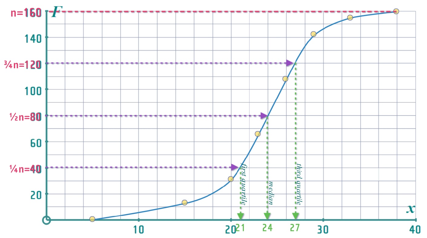
So, the ⲙⲉᕍⲓⲁⲛ \(= 24\) m and the ႳⴑⲀꞄⲦⲒ𝓛ⲈϨ are: \(Ⴓ_{3} = 27\) and \(Ⴓ_{1} = 21\)
Note: Strictly speaking, if \(n = 100\), then the middle 𝑣𝑎𝑙𝑢𝑒 is the \(\frac{1}{2} \left(\color{var(--red)}{100} + 1 \right)\)th-𝑣𝑎𝑙𝑢𝑒 (i.e. the \(50½\)th-𝑣𝑎𝑙𝑢𝑒) - so we should really have looked up \(50½\) on the \(y\)-axis...
...but in practice, when \(n\) is large (> 30) then the difference between using \(\frac{1}{2} \left( n+1 \right) \) and just \(\frac{1}{2}n\) isn't really worth bothering with...
...So, as statisticians, we've all agreed that when \(n \gt 30\), we'll all use \(\frac{1}{2}n\)
We don't use them as much as Americans: Pupils in the \(90\)th ᖘᕮᖇᑕᕮƝƬᓮしᕮ in maths might be put in an advanced programme, whereas those below the \(15\)th ᖘᕮᖇᑕᕮƝƬᓮしᕮ will have to attend SUMMER-SCHOOL instead of having a summer-holiday...
(There's no separate version for \(n \leqslant 30\), because ᖘᕮᖇᑕᕮƝƬᓮしᕮ⟆ are really only used for large ᖙᎯ𝜏ⲁ sets)
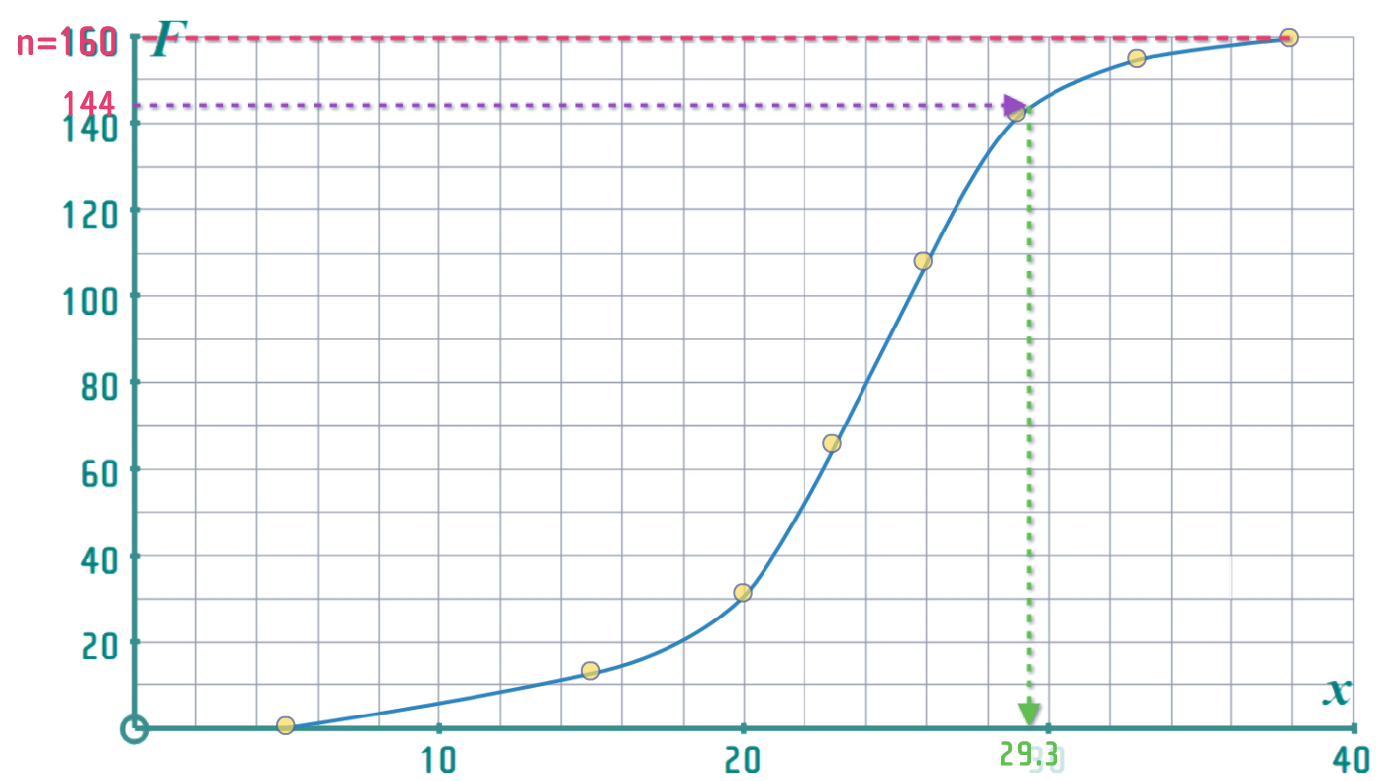
So, \(ᖘ_{90} = 29.3\) m: i.e. if you threw over \(29.3\) m, you were in the TOP \(10 \%\)
The Southern Rail Service's \(8:15\) train to Paddington has been experiencing large delays over the past 3 months.
A survey was taken last month of the amount of time commuters spent waiting for the \(8:15\) train and the results are summarised in the Cumulative Frequency Curve below (you can download it here)
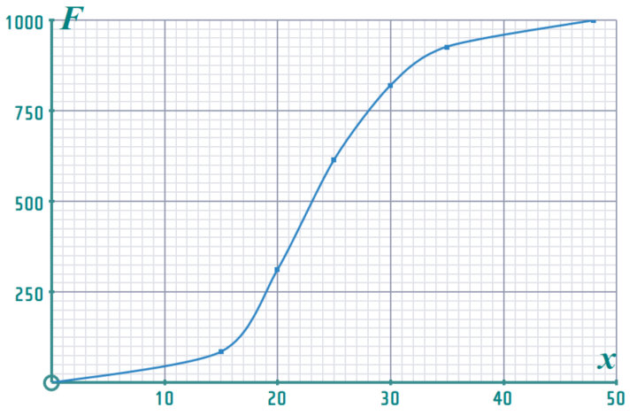
a) From your printout of the curve, estimate* the ⲙⲉᕍ╹ⲓⲁⲛ wait time...
b) State what percentage of customers can expect to wait more that the ⲙⲉᕍ╹ⲓⲁⲛ wait time.
c) From your printout of the curve, estimate* how many of the \(1000\) commuters surveyed waited less than \(30\) minutes for their train
The train company must refund any commuter who has to wait \(30+\) minutes for the train
d) Estimate* how many commuters can apply for a refund?
The regulator will FINE the company \(£2,000,000\) if \(2\%\) (or more) of commuters experienced ❛excessive❜ delays (❛excessive❜ is defined as: 45 minutes or more), raising the fine to \(£5,000,000\) if \(5\%\) (or more) experienced ❛excessive❜ delays
e) How much (\(£0\) if you decide ❛NO FINE❜) will the company be fined?
*Marks will only awarded if your answer is accurate to \(±5\%\) - Print the graph off and be as accurate as you can
Hint
Hints & helpful advice:
Part (a):
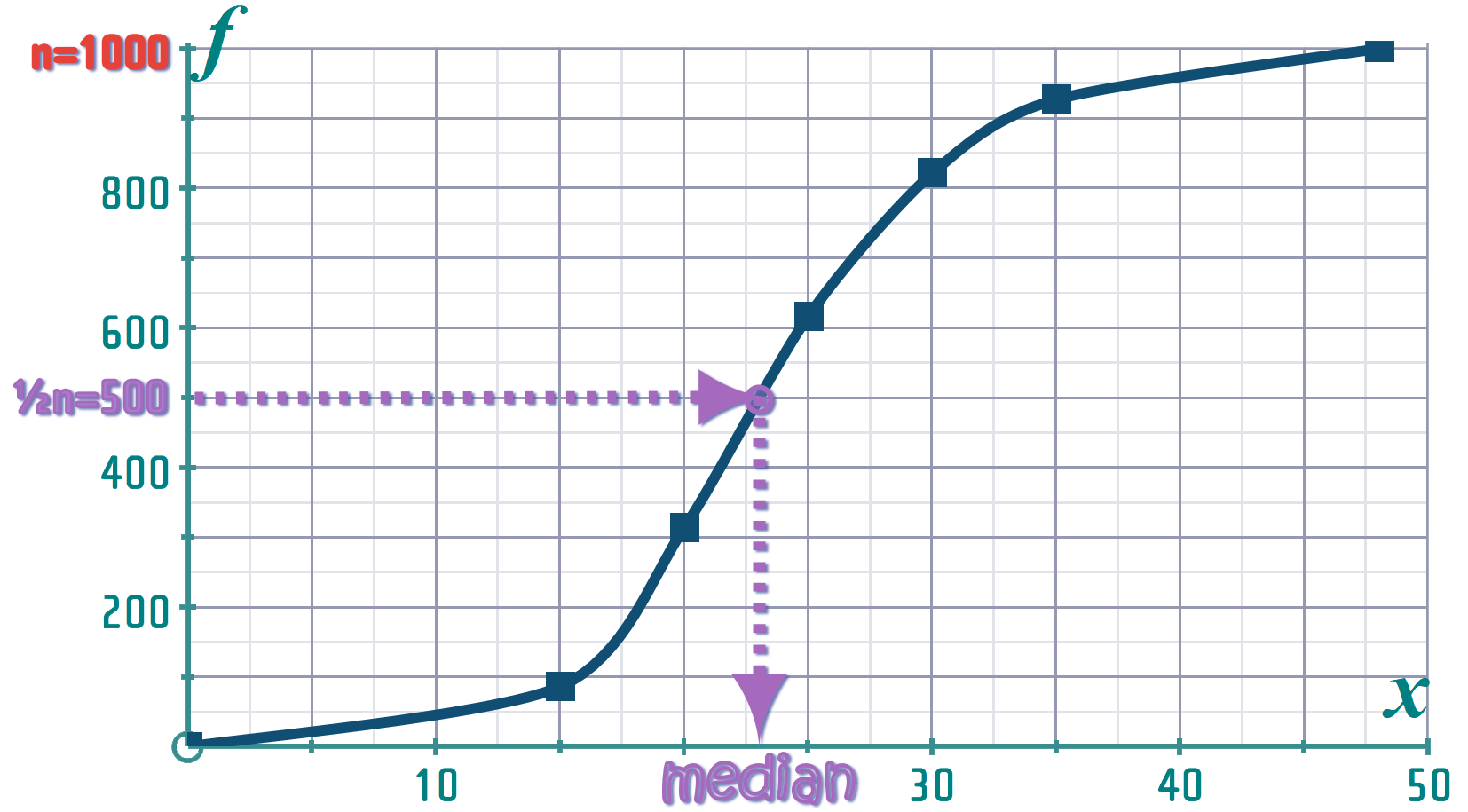
Since \(n=1000\), the ⲙⲉᖙ┊ ⫯ⲁɳ is the \(500\)th value (since \(n>30\), we can use \(\frac{1}{2}n\) instead of \(\left( \frac{1}{2}n + \frac{1}{2} \right) \) )
So, identify \(\frac{1}{2}n=500\) in the \(y\)-axis, draw a horizontal line to the curve, then go vertically down to the \(x\)-axis: Read off the ⲙⲉᖙ┊ ⫯ⲁɳ
Part (b):
The ⲙⲉᖙ┊ ⫯ⲁɳ marks the middle point in the ᖙᎯ𝜏ⲁ: So half of the ᖙᎯ𝜏ⲁ will be values that are below the ⲙⲉᖙ┊ ⫯ⲁɳ, and half of the ᖙᎯ𝜏ⲁ will be values that are above the median...
...always
Part (c):
Firstly - PRINT OFF THE FULL PAGE CUMULATIVE FREQUENCY CURVE for this question…
We want to know how many people waited LESS THAN \(30\) minutes
So, we go to ❛\(30\)❜ on the \(x\)-axis
Add in a vertical line up to meet the curve and then a horizontal line across to the \(y\)-axis
Reading the number from the y-axis tell us how many people waited less than \(30\) minutes
Part (d):
When we read a \(y\)-value from the GRID, it always tells us the NUMBER that were LESS THAN the corresponding \(x\)-value…
If we wanna know how many were MORE than that \(x\)-value, we need to subtract the y-value from ❛\(n\)❜ (remember, ‘n’ is the total number in the sample, which is the LAST number in the cumulative frequencies and also the y-value of the TOP of the ogive…)
Part (e):
Okay, so we wanna know ❛What percentage experienced a delay of \(45\) minutes or more... ❜
So, we go to ❛\(45\)❜ on the \(x\)-axis
Add in a vertical line up to meet the curve and then a horizontal line across to the \(y\)-axis
Reading the number from the y-axis tell us how many people waited less than \(45\) minutes
Since \(n = 1000\), if we subtract that answer from \(1000\), we'll knowe how many waitined more than \(45\) minutes
Finally, to turn that into a percentage, we divide by \(n=1000\) and then multiply by \(100 \%\)
West Coast Railways wish to take over Southern's service - but their own train service to Hogsmeade Station has also suffered some delays. A much smaller sample gave these results:
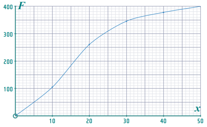
a) From your printout of the curve, estimate* what percentage of these commuters waited \(15-30\) minutes for their train?
b) Estimate* how many of the \(400\) commuters surveyed waited \(30+\) minutes for their train.
Comment on whether - based upon this criterion - West Coast Railways would be better at operating the service to Paddington, or not?
The regulator will also consider the number of excessive delays, before deciding if Southern should be stripped of the franchise...
c) Compare the ᖙᎯ𝜏ⲁ on excessive delays between the two companies: Which company looks better on this metric?
*Marks will only awarded for accuracy \(±5 \%\) - print the graph off and be as accurate as you can
Hint
Hints & helpful advice:
Part (a):
If we draw a vertical line at \(x = 30\) minutes and read across to the \(y\)-value - that will tell us how many passengers waited LESS THAN \(30\) minutes
If we draw a vertical line at \(x = 15\) minutes and read across to the \(y\)-value - that will tell us how many passengers waited LESS THAN \(15\) minutes
SUBTRACT these two values, and we'll get the number that waited BETWEEN \(15-30\) minutess
How do we then turn that into a percentage?
Part (b):
Since the SAMPLE-SIZES are different, it's wrong to just compare the NUMBER that waited \(30+\) minutes
It makes much more sense to compare the PERCENTAGE that waited \(30+\) minutes
Part (b):
Again, we just need to compare the PERCENTAGES!
The Cumulative Frequency Curve below summarises the ᖙᎯ𝜏ⲁ for the heights of \(4000\) G.C.S.E. students
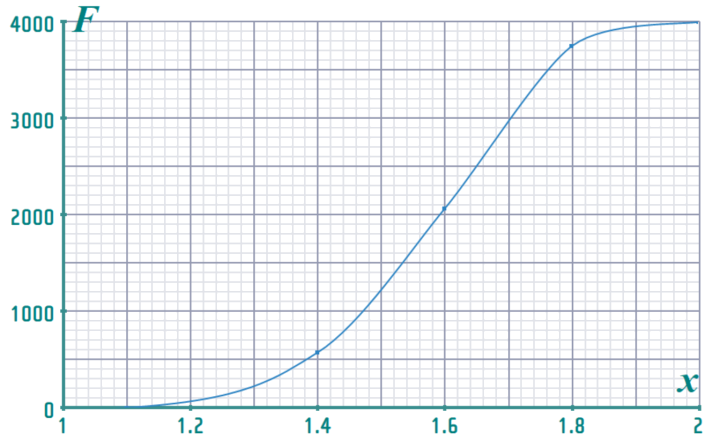
Print off this cumulative frequency curve and estimate*:
a) the percentage of students were between \(1.4\) m and \(1.7\) m tall
b) how many students were exactly \(1.5\) m tall?
c) the height that the tallest \(25 \%\) of students exceeded
d) the height that the shortest \(25 \%\) of students were below
It is decided that students above the \(90\)th ᖘᕮᖇᑕᕮƝƬᓮしᕮ in height should be put on growth supressing hormones to ensure they can still fit through doorways after they become adults.
e) Ayaan is \(1.77\) m tall: By determining the threshold, decide if Ayaan is right to be depressed at the thought that he'll need to be ❛supressed❜
*Marks will only awarded if your answer is \(±5 \%\) of the exact value. So, print the graph to show your workings and try to be as accurate as you can
Hint
Part (a):
Start by finding the NUMBER of students that were \(1.4 - 1.7\) m tall: By drawing vertical lines at \(x=1.7\) and \(x=1.4\), reading across to the \(y\)-values and subtracting…
Then turn it into a percentage (by dividing by \(n=4000\))
Part (b):
This is kinda a ‘trick’ question - but understanding the answer is gonna be crucial to your understanding of continuous ᖙᎯ𝜏ⲁ…
It's not impossible to deduce: If you follow the logic of how you answered Part (a), then it's kind-o-bvious - a ‘prize’ to anyone that gets it right!
Part (c):
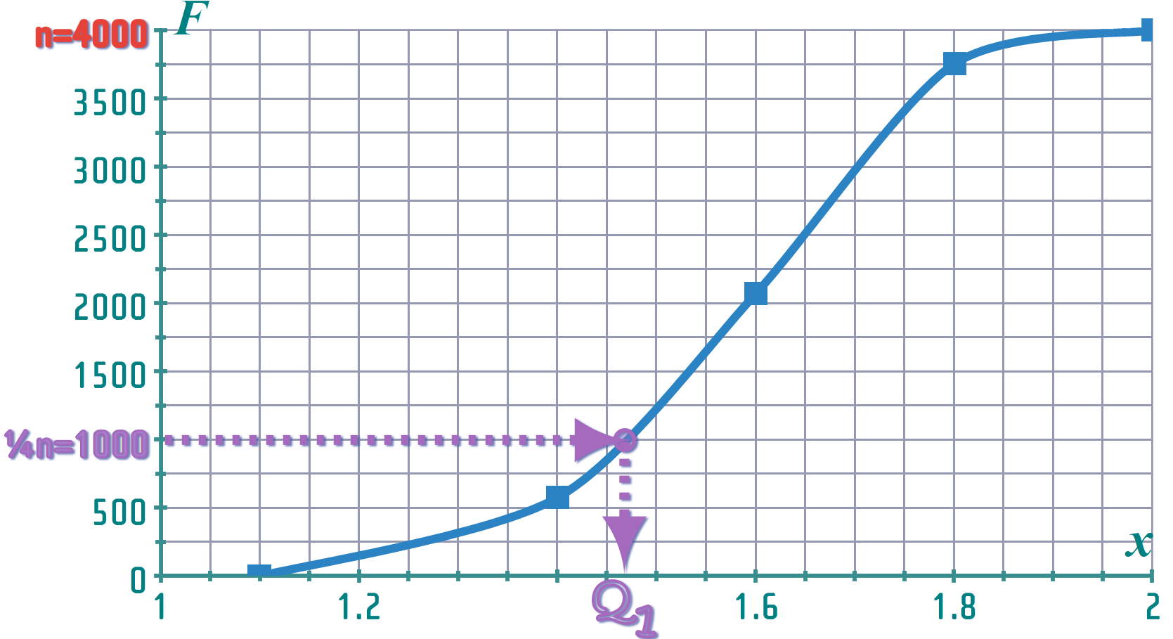
This is actually asking you to find the ⳐOᗯƐᏒ-ႳⴑⲀꞄⲦⲒ𝓛Ⲉ (\(Ⴓ_{1}\))...
Since \(n=4000\), \(Ⴓ_{1}\) is the \(1000\)th-value (since \(n>30\), we can use \(\frac{1}{4}n\) instead of \(\left( \frac{1}{4}n + \frac{1}{2} \right) \) )
So, identify \(\frac{1}{4}n=1000\) in the \(y\)-axis, draw a horizontal line to the curve, then go vertically down to the \(x\)-axis: Read off \(Ⴓ_{1}\)
Part (d):
This is actually asking you to find the ᑌᖘᑭᕮᖇ-ႳⴑⲀꞄⲦⲒ𝓛Ⲉ (\(Ⴓ_{3}\))...
Part (e):
WE are asked to find the \(ᖘ_{90}\) threshold:
In other words, they want to know what height the TALLEST 10% (at the TOP of the curve) all exceed…
 …10% of 4000 is 400
└─────────┬─────────┘
          │
          └────────────  The 400 at the ‘TOP’ of the curve are
                         the 400 between y = 3600 and y = 4000
So if we find the height corresponding to \(y=3600\), this will be the threshold above which all the kids will be given hormone supressants...
Referring back to the ᖙᎯ𝜏ⲁ from QUESTION 1:
A class of \(60\) pupils were asked how much Christmas money they received
The results are given in this table:
Find the ⲙⲉᕍ╹ⲓⲁⲛ and the 𝕀ƝƬⲈꞄ𝓠ⴑⲀꞄⲦⲒ𝓛ⲉ-ꞄⲀⲚᎶⲉ for these ᖙᎯ𝜏ⲁ
Hint
Hints & helpful advice:
We already know that \(n = 60\) (i.e. the total number in the sample was 60)
The ⲙⲉᖙ┊ ⫯ⲁɳ is the \(30\)th-value (since \(n>30\), we can use \(\frac{1}{2}n\) instead of \(\left( \frac{1}{2}n + \frac{1}{2} \right) \) )
So, identify \(\frac{1}{2}n=30\) on the \(y\)-axis, draw a horizontal line to the curve, then go vertically down to the \(x\)-axis: Read off the ⲙⲉᖙ┊ ⫯ⲁɳ
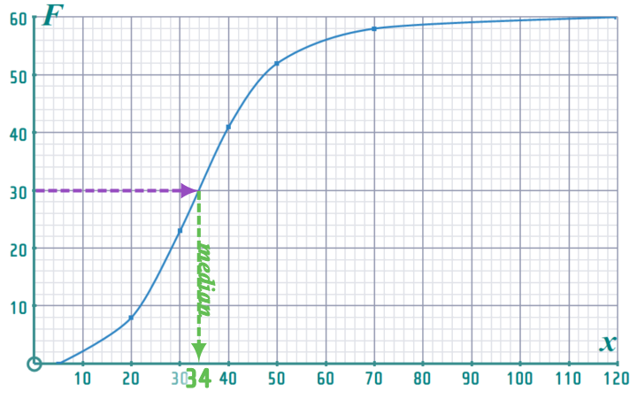
WARNING: ››› Students sometimes write: MEDIAN = \(30\) = \(34\) ‹‹‹ which you should obviously recognise gobbledegook (how and \(30=34\) ???) - it is BETTER to write: MEDIAN (30th value) = 34
Similarly, the \(3^{rd}\) ႳⴑⲀꞄⲦⲒ𝓛Ⲉ is the \(45^{th}\)-value, and the \(1^{st}\)-ႳⴑⲀꞄⲦⲒ𝓛Ⲉ is the \(15^{th}\)-value...
Referring back to the ᖙᎯ𝜏ⲁ from QUESTION 2:
Some ᖙᎯ𝜏ⲁ was collected on the time taken to complete a crossword (with a 2-minute penalty for each incomplete/incorrect entry):
a) Estimate the ⲙⲉᕍ╹ⲓⲁⲛ and 𝕀ƝƬⲈꞄ𝓠ⴑⲀꞄⲦⲒ𝓛ⲉ-ꞄⲀⲚᎶⲉ for these ᖙᎯ𝜏ⲁ
Barry and Sidoni are siblings and they are going to complete the crossword independently of each other
b) What is the probability the both of them complete it it under \(28\) minutes?
Hint
Hints & helpful advice:
Sorry - no help for you here!
Referring back to the ᖙᎯ𝜏ⲁ from QUESTION 3:
Indian airlines tells its passengers that they can "carry on" hand baggage of up to \(10\) kg, but anything above \(10\) kg has to be checked into the hold and the customer needs to PAY for it.
On Tuesday's flight, \(48\) people tried to board the plane with OVERWEIGHT "carry-on baggage"
This table summarises the masses of those idiots:
When ᖙᎯ𝜏ⲁ is grouped like this - it is no longer possible to know the smallest and largest values from the original ᖙᎯ𝜏ⲁ:
In that case, we use \(ᖘ_{10}\) (the \(10\)th ᖘᕮᖇᑕᕮƝƬᓮしᕮ) and \(ᖘ_{90}\) (the \(90\)th ᖘᕮᖇᑕᕮƝƬᓮしᕮ) as representing the where the extreme ends of the ᖙᎯ𝜏ⲁ lie...
b) Estimate* \(ᖘ_{10}\) and \(ᖘ_{90}\) for these ᖙᎯ𝜏ⲁ
c) If two passengers are chosen at random, what is the chance that BOTH will be carrying bags weighing between \(ᖘ_{10}\) and \(ᖘ_{90}\)?
*Marks will only awarded if accurate to \(±5\%\) of the exact value - be as accurate as you can
Hint
Hints & helpful advice:
Firstly, before we can find ⲙⲉᖙ┊ ⫯ⲁɳ/ႳⴑⲀꞄⲦⲒ𝓛ⲈϨ/ᖘᕮᖇᑕᕮƝƬᓮしᕮ⟆ etc we need a 𝓒𝓬𝓾𝓶𝓾𝓵𝓪𝓽𝓲𝓿𝓮-𝓯𝓻𝓮𝓺𝓾𝓮𝓷𝓬𝔂-ᖶᕬᙗᒶᕦ and a 𝓒𝓬𝓾𝓶𝓾𝓵𝓪𝓽𝓲𝓿𝓮-𝓯𝓻𝓮𝓺𝓾𝓮𝓷𝓬𝔂 𝓬𝓾𝓻𝓿𝓮 (remembering to show \(n = 48\) on our curve)
Americans call the MEDIAN the \(50^{th}\)-ᖘᕮᖇᑕᕮƝƬᓮしᕮ (we use: \(\frac{1}{2}\), they use: \(\frac{50}{100}n\) - same difference!)
To find the \(90\)th ᖘᕮᖇᑕᕮƝƬᓮしᕮ, start by working out \(\frac{50}{100}n\)
Then look up this value on the y-axis and read across to the \(x\)-axis
Jack has wants to become 'hench'
He's started doing weights - but, because he's 'ᖙᎯ𝜏ⲁ focussed', he's been examining how much the other guys at the gym are able to bench-press. Here's his ᖙᎯ𝜏ⲁ:
a) Is this ᖙᎯ𝜏ⲁ written using ᙅしᗩ⟆⟆-ᗷ〇⋃Ɲᗩᗪᖇᓮᕮ⟆ or ⊂Լᗩ𝛓Ϩ-し⫯ᵐ𝒾𝜏⟆?
b) Complete this cumulative frequency table
c) Print off this grid and add the O̷G̷I̷V̷E̷ to the grid
From your curve, estimate*:
d) How many gym-guys bench-pressed more than \(45\) kg
e) What the median and the quartiles of the ᖙᎯ𝜏ⲁ are
*Marks will only awarded if accurate to \(±5\%\) of the exact value - be as accurate as you can
Hint
Hints & helpful advice:
This is NOT WRITTEN using ᙅしᗩ⟆⟆-ᗷ〇⋃Ɲᗩᗪᖇᓮᕮ⟆ (this is: ⊂Լᗩ𝛓Ϩ-し⫯ᵐ𝒾𝜏⟆)
                    these should
                    be the same!
                    ┌┬────────┬┐
                    ▼▼        ▼▼
 WEIGHT (kg) │   10-19        20-29        30-34        35-39        40-49        50-59
─────────────┼─────────────────────────────────────────────────────────────────────────
      f      │     7           21           28           32           23            9
The ᙡᕩᙘ ᒹᕩᔜᔚOͦᘉ showed you that, when that happens - you need to consider some values between \(x = 19\) and \(x = 20\) and see which 𝒞ℒ𝒜𝒮𝒮 each value belongs in...
                  ┌─────────────┐                          ┌─────────────┐
  WHICH CLASS:    │ 10 < x ≤ 19 │           OR             │ 20 < x ≤ 29 │
                 ┌┴────┬─┬─┬─┬──┘                        ┌─┴───┬─┬─┬──┬──┴─┐
            ┌────┘ ┌───┘ │ │ └───┐                  ┌────┘  ┌──┘ │ │  └──┐ └────┐
       ┌────┘ ┌────┘  ┌──┘ └──┐  └────┐       ┌─────┘ ┌─────┘ ┌──┘ └──┐  └────┐ └────┐
      19    19.1    19.2    19.3    19.4    19.5    19.6    19.7    19.8    19.9    20
                                           └─┬──┘
                                          ┌──┘
                   ┌──────────────────────┴────┐
                     THIS IS THE CUT-OFF VALUE
                   └────┬──┬───────────────────┘
So we change:           │  │
                     ┌──┘  └──┐
 WEIGHT (kg) │   ⋯-19.5     19.5-⋯         ⋯-⋯         ⋯-⋯         ⋯-⋯         ⋯-⋯
─────────────┼─────────────────────────────────────────────────────────────────────────
      f      │     7           21           28           32           23            9
Next, do the same to every υᖰᕈ∈ᖇ-𝘭⫯ⲙ⫯𝜏 (i.e. add \(\frac{1}{2}\))
Then, do the same to all the ɬσɯҽɾ-𝘭⫯ⲙ⫯𝜏⟆ (i.e. subtract \(\frac{1}{2}\))
Once you've got it written using ᙅしᗩ⟆⟆-ᗷ〇⋃Ɲᗩᗪᖇᓮᕮ⟆, can carry on as usual!